User
Manual for Excel-Macro add_to_contents
Quick Info
Using the
macros add_to_contents and restore_contents_table you can generate a table of
contents for an Excel file. Then you can move very quickly to the cells which
you want to see, instead of scrolling through multiple worksheets, rows and
columns.
add_to_contents: Add selected cell to the table of contents.
restore_contents_table: Add cells with cell names to the table of contents.
Example:
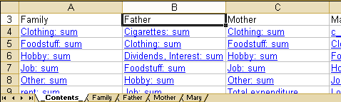
Table of Contents
Searching a location in the file
DIFFERENT_COLUMNS_FOR_EACH_WORKSHEET
Table of Contents from Different
Files
Various Categories for the Headlines
Display Cell Name instead of Cell
Text
Introduction
Microsoft
Word (and other text writing programs) offers a function to generate a complete
contents table with a few mouse clicks. Why is there no such function in Excel?
In Excel you even cannot defines headlines that could be used for generating a
table of contents. This could be changed easily, but there would remain some
other problems. A Word file is mainly a linear document (exemptions are tables
etc.). This means that the order of the contained objects (words, pictures,
etc.) is from top to bottom. Such an order is required to generate a table of
contents in the common sense.
Excel,
however, contains data (text, numbers, diagrams, etc.) within cells, which are
ordered from top to bottom as well as from left to right. Also there are
multiple worksheets within a single file. It seems that it was too difficult
for the Microsoft programmers to build a function to generate a table of
contents from this data. So I have done it and you can obtain a table of
contents that looks like this:
This file
is a simple cash journal for a family which wants to keep an overview about
there income and expenditures. There is a worksheet for each family member. The
table of contents is produced with following parameters (adjustment of
parameters, see below):
- For each worksheet a column is
generated.
- The entries are sorted
alphabetically by the displayed text
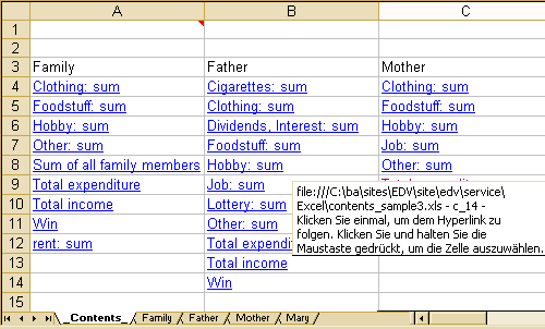
- Each entry is a hyperlink. The
destination is displayed, if you move the mouse pointer over this
hyperlink. Clicking the hyperlink will cause Excel to move to the
destination cell.
Installation
How to
install this macro and how to define a shortcut key combination for running the
macro, you can read on my page Excel Makros.
Using
the macro
Select the cell
which you want to add to the table of contents and then start the macro. That’s
it.
If you
select multiple cells, all selected cells are added to the contents.
How the
table of contents should look like, you should adjust once before using the macro.
May be you
will need an expert to install the macro and adjust the settings. But after
this is done, using the macro is very easy.
Using
the Table of Contents
Searching
a location in the file
Of course,
you may print the table of contents. The most important function, however, may
be, that you rapidly can jump to a certain location in the file just by
clicking the entry in the contents. Especially in large files with many
worksheets and a lot of rows and columns, this may save plenty of time.
Invalid
Links
If you
click onto an entry in the table of contents and Excel prompte a message that
the link is invalid,

this may be
caused, that you have deleted the referenced cell, as Excel deletes the name of
cell too, if the cell is deleted. In such a case you should remove the entry
from the contents manually.
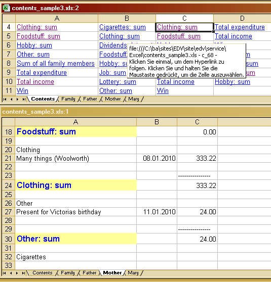
Working
with 2 Windows
This is for
most efficient working. Assuming you want to update your family’s cash journal
and you have a list of income and expenditures to insert. Open a second window
using the entry Window in the Excel
menu bar and select New Window. Then
Excel creates a second window for displaying the same file. (You can see this,
as Excel shows :2 or :1 behind the filename in the title bar.) Now put the both
windows side by side, or one above the other and select the worksheet with the
table of contents in the second window. If you click onto an entry, the first window
jumps to the referenced cell und the second window continues showing the
contents. This save a lot of work compared to the case that you would move
yourself through the multiple worksheets.
Deleting
Entries
If you want
to delete an entry of the table of contents, you can just delete this cell.
Please note, that there will remain no empty cell in the middle of a column of
the table of contents, as an empty cell would tell the macro the end of the
entries in this column. New entries would be inserted afterwards at a wrong
location. Therefore it is important that you delete the complete cell and not
only the content of the cell! When deleting the cell, Excel asks you what
should happen with the other cells. If you select move upwards (the cells below, but not the complete rows), the gap
at the deleted cell will be filled properly.
Deleting an
entry of the table of contents will not change the format of the referenced
cell! This cell continues to look like a cell that was inserted into the
contents until you will change the format manually. A macro cannot do this job,
as it does not know how the cell looked like before adding it to the contents.
Changing
Excel Data
If you want
to change Excel data after generating the table of contents, you should pay
attention to the following points:
- If you used USE_NAME_FOR_REFERENCING = 0, the macro used the actual address
(row, column, name of worksheet) of the cell to generate the hyperlink for
the table of contents. If you insert a new line above this cell, the row
number of the cell is changed. Unfortunately, Excel does not update the
hyperlink and this will become an reference to another cell. You will have
the same problem, is you change the name of the worksheet. Then Excel will
prompt a message Invalid Link,
as the original name no longer does exist. Using USE_NAME_FOR_REFERENCING = 1, these errors will not occurr.
- If you delete cells, which have
been added to the table of contents, the names of these cells will be
deleted too and the link in the table of contents becomes invalid and
should be removed manually.
- If you copy cells which have
been added to the table of contents, the format is copied too and, seeing
the format of headlines, you may think that this cell is contained in the
contents. But this is not true. Excel even does not copy the name of cells
when the cell is copied! So you should add those cells to the contents
yourself. Or, if you do not want this, change the format to look like
normal cells.
- This is different, if you copy
a complete worksheet. In this case, Excel copies the cell names too (and
internally puts the worksheet name in front of it to avoid double names).
Those copied cells are not inserted in the table of contents, but you can
do this using the Macro restore_contents_table.
Settings
The look of
the table of contents can be adjusted using some Const-parameters, which are
contained at the top of the macro file. Using the description below, it should
be possible for normal computer users to do these settings themselves. The
function and the possible values of the parameters are explained here. For
editing these parameters you must open the source code of the macro. Open the
list with the installed macros using the function key Alt-F8. Then select the macro add_to_contents
(no double click, as it would start the macro) and click the button Edit. This opens the macro editor. If it
does not work, you may have no license to do it.
It may be
useful to make a copy of the complete macro text and save it in a simple text
file. Then it will be easy to restore the original program code.
It is also
possible to work with comments. Copy the line, which you want to change.
Inserting a “’” at the beginning of the original line tells the program not to
use this line. Then you can modify the copied line and text. If everything
works well, you can save the macro by clicking the save-symbol.
Common
Parameters
WS_CONTENT_NAME
This
parameter tells the name (enclose it within double quotation marks) of the worksheet,
into which the table of contents will be written. If this worksheet does not
exist, it will be generated at the first call of the macro.
Every time
the macro is called, it looks for a comment of the cell at the very top left
(row 1, column A). If there is no comment, the macro adds one and will store
there the number of entries that have been inserted into the table of contents.
Do not change this number yourself without having understood how the macro
works, as the macro will use it to generated unique cell names.
If you
want, you may store other data in the contents worksheet too, but you should
avoid that the table of contents overlaps with your data! When inserting a new
entry, the macro may move down all the cells in the column (starting at the
insertion row) by one row. This could destroy the order of your data, if there
are any, in this column below the START_ROW.
If you
enter ACTUAL_WORKSHEET for this parameter, a table of contents is generated at
the top of each worksheet, but this table of contents only contains the entries
of this special worksheet. So every worksheet will get its own contents. You
must ensure that there is enough empty space for the table of contents.
START_ROW,
START_COLUMN
START_ROW is the line number where the table of contents
starts. If a column headline is generated, this is written into START_ROW – 1.
Therefore START_ROW should be at least 2. The upper border depends on the
version of your Excel.
START_COLUMN is the column number where the table of
contents starts. It must be at least 1, the maximum depends on the version of
your Excel.
SORTING
There are 4
valid values for sorting to determine how the entries within one column of the
table of contents are sorted:
- 0: No sorting. New entries are
added below the last entry in the column.
- 1: Sort by the displayed text.
This is the text of the cell which is to be added to the table of
contents. If this cell contains a formula, the displayed text will not be
the formula itself, but the result of the formula.
- 2: Sort by the row number of
the referenced cell. In case of equal row numbers, the column number is
used as second sorting condition.
- 3: Sort by the columns number
of the referenced cell. In case of equal column numbers, the row number is
used as second sorting condition.
ADD_WORKSHEET_NAME
- 1: Insert the name of the
worksheet in front of the displayed text of the cell. The advantage is,
that you can see immediately to which worksheet the link refers.
Especially if all the table of contents is print to a single column, this
could be helpful. The disadvantage is, that the displayed text becomes
longer and a part of the displayed text could be hidden if the column
width is too small.
- 0: Display text without
worksheet name
DIFFERENT_COLUMNS_FOR_EACH_WORKSHEET
- 0: The macro writes all entries
of the table of contents into a single column (START_COLUMN).
- 1: The macro generates an own
column in the table of contents for each worksheet. The name of the
worksheet is written into row START_ROW – 1. The order in which the
columns are generated is the order in which you add entries of the various
columns. Note that there are enough columns for the table of contents!
(Old Excel versions are limited to just 256 columns.)
ADD_NAME_FOR_THE_CELL
In Excel
you can assign names to single cells or areas of cells. Then you can work with
these names instead of using the addresses. For example, in formulas you may
use the cell names instead of the addresses. Then you can immediately see the
meaning of the cell.
The macro
uses cell names to mark the cells that are added to the table of contents. With
this information the macro restore_contents_table
can restore the complete table of contents, if you set ADD_NAME_FOR_THE_CELL to
3, 4 or 5. This may be useful, if you have deleted a lot of cells.
Terminology:
content-counter-name
A cell name
of format c_xxxxx, where xxxxx is a 5 digit number. Such names are generated by
the macro.
content-name
A cell name
starting with “c_” (a lower case letter c followed by an underscore). Such
names may be defined for cells by the user, if he wants to mark them for the
table of contents, as the macro restore_contents_table will find such names and
is able to distinguish them from other names.
cell-name
Any name
that has been defined for a cell (by user or macro).
- 0: The cell does not obtain a
name.
- 1: The displayed text of the
cell becomes its name.
- 2: Same as 1, but only if the
cell does not have another name.
- 3: The cell is named by a content-counter-name of the format
c_xxxxx, where xxxxx is a 5 digit number with leading zeroes (for better
sorting in the Excel name list) of the number of entries which have been
added to the table of contents. (This number is saved in the contents
worksheet cell A1.)
- 4: Same as 3, but the content-counter-name is assigned to
the cell only, if the cell does not have already a content name. (Names, which do not match the content name format, are ignored
her.) Usually, this setting will be the optimum one.
- 5: Same as 3, but all existing content-counter-name for this cell
are deleted before assigning the new content-counter-name.
Mostly, this method makes no sense, as the existing hyperlinks would
become invalid and AVOID_DOUBLETS = 1 will no longer work. But the macro restore_contents_table uses this
setting, if you click onto „Yes“ in the message box appearing after its
start.
ADD_WS_TO_CELL_NAME
This is an
additional parameter for the generation of the cell name (see ADD_NAME_FOR_THE_CELL).
1: The name
of the worksheet is added in front of the cell name. This may be useful, it
there would exist equal cell names in different worksheets.
0: The name
of the cell does not contain the name of the worksheet.
USE_NAME_FOR_REFERENCING
Excel
offers two possibilities for defining a hyperlink to a cell:
- 0: Referencing the cell by its
address. In this case the link becomes wrong, if the address of the
referenced cell changes (e.g. by insertion or deletion of cells).
- 1: Referencing the cell by its name. In this case the link remains well even after insertion or deletion of other cells. But this requires the cell having a name (see ADD_NAME_FOR_THE_CELL). Mostly, this will be the better setting.
TEXT_TO_DISPLAY
The text
that is displayed in the table of contents for the selected cell
- 1: cell text as displayed in
the selected cell
- 2: cell name (entered by the
user or automatically). If there is no cell name, method 1 is used
instead.
- 3: cell name, if it is not a content-counter-name, cell text
else. What is the sense of this setting? If there are cells which show a
meaningful text, this text is displayed in the table of contents and the
macro will assign a less meaningful content-counter-name
to the cell, if you do not define a name for this cell. But for cells,
that only display numbers, a meaningful name will be displayed if you
define such a name. So this setting may be helpful to work with a mixture
of text and numerical cells.
AVOID_DOUBLETS
- 1: The macro avoids double
links to a single cell. If the macro sees that there is already another
link to the selected cell in the table of contents, it does not add a new
entry.
- 0: The macro adds the new entry
without performing the doublet test.
MARK_CELL
The macro
can mark the cells, which you add to the table of contents. Then you can see
easily, which cells are already contained in the contents.
- 0: No mark.
- 1: Add the cell name (see ADD_WS_TO_CELL_NAME) as comment of the cell. Usually the cell comment is shown as a
small red triangle in the upper right corner of the cell. If you move over
it with the mouse pointer, the comment text is displayed. The advantage of
this method (compared to method 2) is that the format of the cell is not
modified. Conflicts may raise, if you want to use the comments for your
own purpose.
- 2: The cell is marked by
changing some format parameters (Font-Parameter). After changing the format,
there is no way (but the manual one) to restore the old format, as Excel
cannot undo changes that have been made by macros. The big advantage is,
that you immediately can see, which cells are already contained in the
contents.
Font-Parameters
The font
parameters are used only, MARK_CELL is set to 2. If
any of the following parameters is negative, this special font property is not
changed. So you can change just the font properties which you like, e.g. it may
be sufficient for you, just to change the background colour of those cells, but
not to change the script type and size.
BACKGROUND_COLOR
This is the
background colour of the cell. Valid are all values of the Excel colours.
Sample: 36 is a light yellow. A negative value will cause no change.
FONT_COLOR
This is the
colour of the letters. Valid are all values of the Excel colours. Sample: 5 is
blue. A negative value will cause no change.
FONT_NAME
This is the
name of the font for the text in the cell. This parameter is no number, but a
string, which must be included in double quotation marks. Samples are
"Arial", "Times New Roman", "Courier", … An empty
string "" will cause no change.
FONT_SIZE
This is the
font size. For normal cells, mostly 10 or 12 are used. For headlines a larger
value makes sense. A negative value will cause no change,
FONT_UNDERLINED
How to
underline the cell text. Here the following Excel constants should be used:
xlUnderlineStyleNone:
no underline
xlUnderlineStyleSingle:
single underline
xlUnderlineStyleDouble:
double underline
Missing
Features
You have
seen that the macro can perform several useful tasks for you. Of course, there
is a lot to be improved. If you need anything, I may do it for you in exchange
for any type of reward.
Table
of Contents from Different Files
In some
cases it would be desirable to generate a table of contents, which is able to
work with cells of different files. It is not really difficult, but the
implementation takes plenty of time for the management of the files, which may
be closed or even no longer existing, or moved to another place, ...
Various
Categories for the Headlines
In
Microsoft Word there are multiple categories for the headlines (headline 1,
headline 2, etc.) in order to obtain a well structured text and table of
contents. The macro add_to_contents actually knows only a single headline
category.
Display
Cell Name instead of Cell Text
Assume you
have a cell containing any formula resulting in a number. If you add this cell
to the table of contents the displayed text will be the resulting number.
Macro restore_contents_table
Using the macro
restore_contents_table you can restore a table of contents. This works only, if
you assigned content-names to the
cells, when they have been added to the table of contents (ADD_NAME_FOR_THE_CELL with values 3, 4 or
5.) or yourself by manual input. After starting the macro, the following
message box will appear:
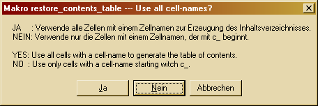
The restore macro reads all
cell-names
of the actual Excel file and calls the macro add_to_contents for all names (in
case of answer “Yes” / “Ja”) or only for those names, which match the content-name
format (in case of answer “No” / “Nein”). If you delete the old table of
contents (or may be move it to another worksheet), a completely new and actual
table of contents is generated. If the macro finds names that became invalid
(e.g. due to deletion of the referenced cells), those names are ignored and no
entry is added to the contents.
The restore macro uses all
the settings of macro add_to_contents with a single exception: For
ADD_NAME_FOR_THE_CELL the values 0 or 5 are used, depending on the button onto
which you will click in the message box appearing immediately after starting
the macro:
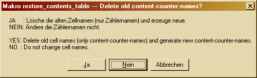
If you click „Yes“ (German
„Ja“), all existing content-counter-names are deleted (but
not the other names!) and are replaced by new content-counter-names. If the
old cell names have been used in any way (links, formulas) this will cause
invalid links. Therefore you should select “Yes” only in the case that you used
the content-counter
names only for the table of contents. Then you will get a new numbering
without gaps. Avoiding doublets (AVOID_DOUBLETS = 1) does not work here, as the
old links become invalid when deleting the old names. Therefore this function
is only good for generating a new table of contents.
For the common user “No”
(German “Nein”) will be better in most cases as this does not change so much.
In any case it makes sense
to make a copy of the complete Excel file before using this macro!
NOTE: This is a simple
possibility to modify the format of the cells which have been added to the
table of contents, or to change the displayed link texts, if the text of the
referenced cells changed.
NOTE: Sometimes it could be
useful, if macro restore_contents_table could work with the cell comments or
the format of the cells for the table of contents. This was not implemented as
comments and formats are organized on the level of cells and the macro would
have to loop through all cells of all worksheets of the workbook.
Version
History
This manual
always belongs to the latest version!
1.0: First
Version, November 2010
Downloads
Here are
some files for downloading. Please note that Excel macros are programs, which
may do many things you wouldn’t like. Be cautious, if you do not know me
personally! Depending on the settings of your computer you may get warning
messages from you download manager, antivirus program or from Excel.
Therefore I
offer the source code as a simple TXT-file, that is less harmful than the page
you are just reading. You may view it in your Browser by clicking onto the
filename or directly download it.
|
File |
Description |
|
Source code of the macros for viewing in browser or
downloading. The parameters are set so that you can create a
table of contents immediately after installing the macro restore_contents_table, if your
file contains cells with names. When you run this macro for testing, click
“Yes“ in the first message box and „No“ in the second one. Test this macro
with a copy of your file! |
|
|
Excel sample file without macros. |
|
|
Excel sample file with macros. |
Copyright
These macros
may be copied, used and modified freely for private and other not commercial
purpose. You may give them or parts of them freely to others only together with
the information about the author, the exclusion of liability and the copyright.
These macros or parts of them must not be sold and they must not be used for
commercial purpose without permission of the author. For this you need a
license (contact) after testing the macro for your purpose for
a maximum of 2 weeks.
Denial
of Liability
The user of the macros is
alone responsible for the results, I herewith deny any liability of my person!
These macros can contain program errors. Many macros overwrite the content of
special cells. This content is lost, as the execution of macros cannot be
undone.
Tip: Test new macros with a sample file. Save the file before executing
a macro. Then the file can be reloaded, if the result was bad.
Responsible:
Bernhard Abmayr, www.edv-abmayr.de, Last update:
26.11.2010